Gradient Descent - The Algorithm That Teaches Machines to Learn

Imagine you’re blindfolded and placed somewhere on a mountain. Your goal? Find the lowest point in the valley below. You can’t see where you’re going, but you can feel the slope beneath your feet. What would you do?

You’d probably take a step in the direction that feels like it’s going downhill most steeply, then repeat. Step by step, feeling your way down the slope until you can’t go any lower. Congratulations! you’ve just discovered the intuition behind gradient descent, the algorithm that teaches machines to learn.

The Mountain Climbing Analogy

This isn’t just a cute story. Gradient descent literally works this way, except instead of a physical mountain, we’re navigating the landscape of a mathematical function. And instead of finding the lowest physical point, we’re searching for the minimum value of a cost function, a measure of how wrong our machine learning model currently is.

Every time a neural network learns to recognize faces, every time a recommendation system gets better at suggesting movies, every time a self-driving car improves its decision-making, gradient descent is working behind the scenes, taking those careful steps down the mathematical mountain.

The Mathematical Heart

At its core, gradient descent follows a beautifully simple rule. For a function $f(x)$, we update our position using:

$$x_{i+1} = x_i - \alpha \frac{\partial f(x_i)}{\partial x}$$

Where $\alpha$ is our learning rate – essentially how big steps we take down the mountain. But what does this actually mean?

Let’s break it down with a concrete example using the function $f(x) = x^2$.

Finding the Slope

To understand how gradient descent works, we need to understand slopes. The slope at any point tells us which direction is “downhill.”

For our function $f(x) = x^2$, let’s derive the slope (derivative) from first principles:

Consider two points: $(x, y)$ and $(x', y')$ where $x' = x - \delta x$. As these points get infinitesimally close:

$$\begin{aligned} \frac{dy}{dx} &= \frac{y - y'}{x - x'} \\ &= \frac{x^2 - (x')^2}{x - x'} \\ &= \frac{x^2 - (x - \delta x)^2}{x - (x - \delta x)} \\ &= \frac{x^2 - (x^2 - 2x\delta x + \delta x^2)}{\delta x} \\ &= \frac{2x\delta x - \delta x^2}{\delta x} \end{aligned}$$

As $\delta x \to 0$, the $\delta x^2$ term vanishes, giving us:

$$\frac{dy}{dx} = 2x$$

The Algorithm in Action

Now here’s where the magic happens. Our update rule becomes:

$$x = x - \alpha \cdot 2x = x(1 - 2\alpha)$$

Think about what this means:

• If $x > 0$ (we’re on the right side of the parabola), the slope is positive, so we move left
• If $x < 0$ (we’re on the left side), the slope is negative, so we move right
• If $x = 0$ (we’re at the bottom), the slope is zero, so we stay put

The algorithm naturally guides us toward the minimum!

From Theory to Machine Learning

“But wait,” you might ask, “how does this help machines learn from data?”

Great question! Let’s say you have some scattered data points and want to fit a line through them:

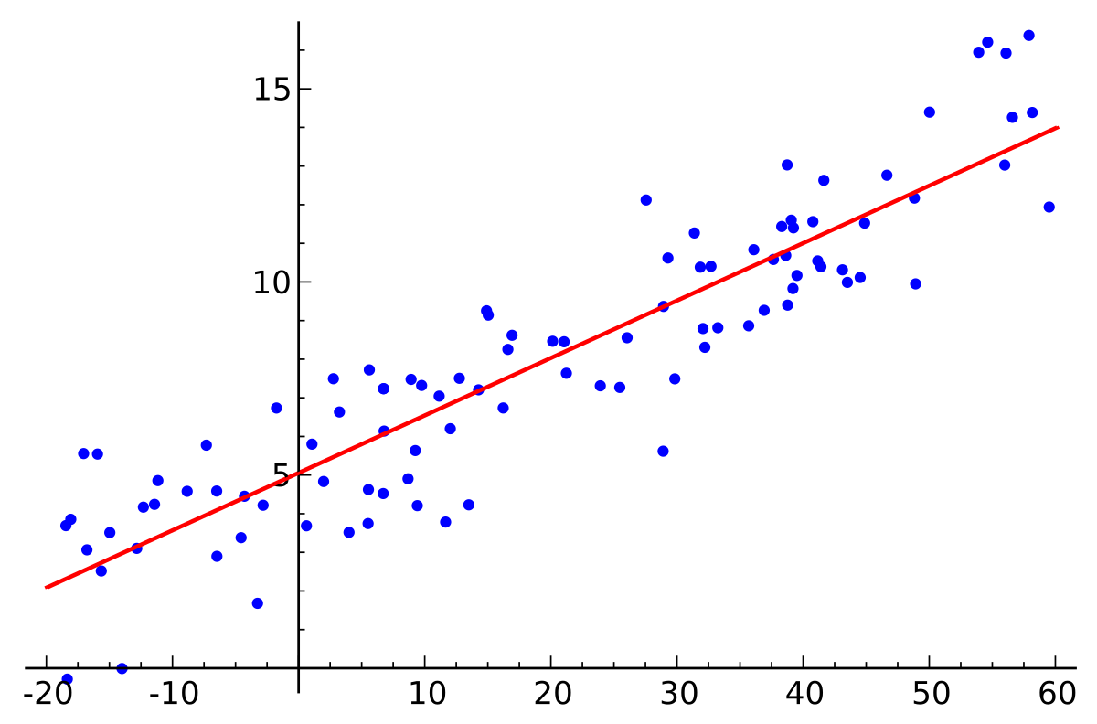
Our hypothesis function $h(x)$ might be a simple line: $h(x) = \theta_0 + \theta_1 x$

But how do we find the best values for $\theta_0$ and $\theta_1$? We need a way to measure “how wrong” our line is.

The Cost Function

We define our cost function as the sum of squared errors:

$$J(\theta_0, \theta_1) = \frac{1}{2m} \sum_{i=1}^m [y_i - h(x_i)]^2$$

This function creates a landscape where the “height” at any point $(\theta_0, \theta_1)$ represents how badly our line fits the data. Our goal? Find the lowest point in this landscape.

The Learning Process

Now we can apply gradient descent to find the optimal parameters:

Repeat until convergence:

$$\begin{aligned} \theta_0 &= \theta_0 - \alpha \frac{\partial J}{\partial \theta_0} \\ \theta_1 &= \theta_1 - \alpha \frac{\partial J}{\partial \theta_1} \end{aligned}$$

Each iteration adjusts our parameters to reduce the cost function, gradually improving our model’s predictions.

The Critical Choice: Learning Rate

The learning rate $\alpha$ is perhaps the most crucial hyperparameter in gradient descent. It’s like choosing how big steps to take down the mountain:

The Goldilocks Problem

• Too small ($\alpha$ too low): You’ll eventually reach the bottom, but it might take forever. Your algorithm crawls down the mountain at a snail’s pace.
• Too large ($\alpha$ too high): You might overshoot the minimum entirely, bouncing back and forth across the valley like a pinball, never settling down.
• Just right: You reach the minimum quickly and efficiently.

Variants and Modern Improvements

The basic gradient descent algorithm has evolved significantly:

Batch vs. Stochastic vs. Mini-batch

• Batch Gradient Descent: Uses all training data to compute each step. Stable but slow for large datasets.
• Stochastic Gradient Descent (SGD): Uses one random sample at a time. Fast but noisy.
• Mini-batch: Uses small batches of data. The sweet spot between stability and speed.

Advanced Optimizers

Modern machine learning employs sophisticated variants:

• Momentum: Adds “inertia” to help roll through small hills and valleys
• Adam: Adapts the learning rate for each parameter individually
• RMSprop: Adjusts learning rates based on recent gradient magnitudes

These improvements help overcome common challenges like getting stuck in local minima or dealing with saddle points in high-dimensional spaces.

Why This Matters

Gradient descent isn’t just an academic curiosity but the engine that powers the AI revolution. Every time you:

• Get personalized recommendations on Netflix
• See your photos automatically organized by faces
• Use voice recognition on your phone
• Experience machine translation

You’re witnessing gradient descent at work, iteratively improving models through countless tiny steps down mathematical mountains.

The Beauty of Simplicity

What makes gradient descent so remarkable is its elegant simplicity. The core idea, following the steepest downhill path, is intuitive enough for anyone to understand, yet powerful enough to train neural networks with billions of parameters.

It’s a perfect example of how the most profound algorithms often emerge from the simplest insights. Sometimes, the best way to solve a complex problem is to break it down into many small, simple steps.

The next time you interact with an AI system, remember: somewhere in the background, gradient descent is quietly taking those careful steps down the mountain, making the system just a little bit smarter with each iteration.